This is a real-time 3D scanning with Xbox Kinect at the beach in Oregon, by James Dietrich and Mark Fonstad. The device projects an infrared pattern (see this other video) and by looking at that pattern reflected on the real objects it calculates the distance for each pixel, in real time. In this case, I am the 'real object', besides the camera holder. This information allows the computer software to 3D rotate the object in the screen in real time (while the object moves, for instance), changing the perspective.
The potential applications for geoscience are... infinite! For example: no need to measure and count pebbles any more, you river geomorphologists, just a 2-second scan and there it comes your grain-size distribution!
And this is a group 3D-picture he took at the same Bretz Meeting in Oregon, last week:
http://youtu.be/s4B3O50q9nk
Amazing, ha? It's a 3D model based on a series of pictures taken with a normal camera.
Update:
Follow this link to learn more technical details about the device.

2012-03-22
Ideas on open questions in Earth Science?
[PD: The result of this initiative is in this later post]
Searching for Unknowns consumes most of our research time and also makes the bulk of our research motivation. Wouldn't it be good to share the biggest open questions in our respective disciplines?
Searching for Unknowns consumes most of our research time and also makes the bulk of our research motivation. Wouldn't it be good to share the biggest open questions in our respective disciplines?
I'm thinking of specific problems that are well established from a scientific point of view and that have an impact on at least a couple of subdisciplines. Examples would be: "What caused the Permian extinction?" or "What drives magnetic polarity reversals?" or "How much of the current climate change is anthropogenic?". But a bit more of elaboration and a key reference would be desirable.
I will try to summarize the compiled ideas in a later entry in this blog, but key references discussing each subject are welcome. I'm looking forward for suggestions or feedback, either as comments to this post (below) or at @danigeos on Twitter.
Update:
Alexandra Witze shares links (in a comment below) to the following relevant documents: 1, 2. Some of the questions summarized there will be useful as a general frame to what i aim at (they are big trans-scientific goals). But I would like to find the top key questions at a more detailed level, more specific, even if of interest only to a minority of subfields within Earth Sciences. Open problems that most assistants to the AGU, EGU, GSA or INQUA meetings could be curious about even if only a small percentage could really judge critically.
Update 2:
A reference to a key paper on the problem proposed will make every contribution much more valuable!
Update 3:
The result of this initiative is in this later post:
2012-03-15
Seafloor spreading, magnetic reversals, and plate tectonics
Doing science consists of formulating refutable hypotheses, this is, new interpretations based on former experience that lead to predictions that can be either confirmed or falsified (by future research).
A case history in Earth science is the confirmation of the plate tectonics theory during the 60's. Back in 1912, this theory was just a hypothesis known as continental drift and put forward most remarkably by Alfred Wegener, based on observations of the fossil fauna matching across different continents. Well, in addition to the matching coastlines of continents pointed out by Abraham Ortelius as early as in the... 16th century!
One implication of the continental drift idea was that the oceans laying between continents that drifted away from each other should have gradually spread apart. This is known as the seafloor spreading hypothesis. But how to prove it?
Much earlier than that, the Earth's magnetic field had been studied scientifically since the beginning of the Spanish and Portuguese explorations of the Americas (Alvarez & Leitao, 2010, Geology, The neglected early history of geoscience). By the 17th century, maritime trading was dependent on the accurate mapping of magnetic intensity across the Atlantic Ocean. These studies culminated by the 19th century during the so-called Magnetic Crusade, leading to the realisation that the magnetic poles migrate significantly over historical time periods. And in fact, these rapid changes of the magnetic field soon became one of the theories proposed to explain why the magnetic orientation recorded in rocks depends on their geological age.
Today we know that historical magnetic changes are normal in periods of stable magnetic polarity, and that although the polarity flips recorded in rocks take just a few thousand years, they occur only over geological time-scales (millions of years).
Back in 1957, Marie Tharp found enigmatic alignments in the shape of the seafloor around the center of the Atlantic Ocean, roughly where seismicity was being detected. In 1963, both the geophysicist Frederick J. Vine and the geologist Lawrence W. Morley independently realized that if the seafloor spreading theory was correct, then the rocks surrounding mid-oceanic ridges should show symmetric patterns of magnetization reversals, recording the changes of the Earth's magnetic field in the volcanic rocks at the time when these erupted and cooled down at the mid-ocean ridges. This is now known as the Vine–Matthews–Morley hypothesis, and became a validation test for the seafloor spreading, and for the plate tectonics theory in general.
Morley's letters to Nature (February 1963) and to the Journal of Geophysical Research (April 1963) were both rejected, so Vine and his advisor Matthews were first to publish the hypothesis on the same year. The patterns of ancient reversals of the Earth's magnetic field have been found thereafter in hundreds of paleomagnetic surveys, providing a robust validation of their hypothesis. In fact, a vast later work of age calibration of these magnetic reversals allowed for the detailed maps of the age of the oceanic floor that we have nowadays:
Magnetic reversals are still today one of the key methods allowing rock dating (don't miss the name for it: magnetochronostratigraphy). But we know very little about the mechanisms responsible for these magnetic field changes. Computer simulations suggest that it is a natural result of feedback forces between the magnetic field and the flow in the Earth's core (see the reference to Glatzmaiers' below), similar to dynamo going tilted by its own magnetic field. It has been recently shown in this article in GRL a correlation between the distribution of tectonic plates and the frequency of magnetic reversals over geological time ("geological intervals characterized by an asymmetrical distribution of the continents with respect to the equator are followed by intervals of high reversal frequency"), suggesting a mechanical coupling between both phenomena. But the specific mechanism behind magnetic reversals and the additional information they may contain about the interior and the past of our planet remain, so far, a challenge (yet another Reto Terrícola!).
Update (2015-09): A Science News article on a recent study on core convection and the magnetic field.
References:
Vine, F., & Matthews, D. (1963). Magnetic Anomalies Over Oceanic Ridges Nature, 199 (4897), 947-949 DOI: 10.1038/199947a0
Pétrélis, F., Besse, J., & Valet, J. (2011). Plate tectonics may control geomagnetic reversal frequency Geophysical Research Letters, 38 (19) DOI: 10.1029/2011GL048784
Glatzmaiers, G., & Roberts, P. (1995). A three-dimensional self-consistent computer simulation of a geomagnetic field reversal Nature, 377 (6546), 203-209 DOI: 10.1038/377203a0
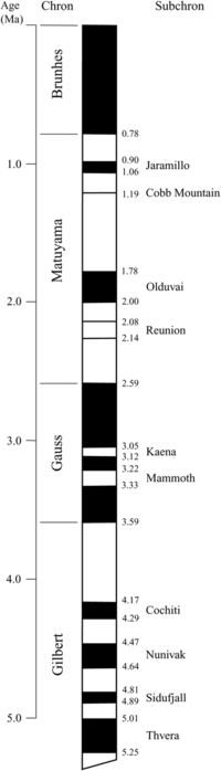 |
Timing of the last reversals of the Earth's
magnetic field. Time goes from 5 Million years ago (bottom) to present (top).
Periods in black match today's polarity;
Source: Wikimedia Commons. A more complete scale here.periods in white underwent reversed polarity. |

One implication of the continental drift idea was that the oceans laying between continents that drifted away from each other should have gradually spread apart. This is known as the seafloor spreading hypothesis. But how to prove it?
Much earlier than that, the Earth's magnetic field had been studied scientifically since the beginning of the Spanish and Portuguese explorations of the Americas (Alvarez & Leitao, 2010, Geology, The neglected early history of geoscience). By the 17th century, maritime trading was dependent on the accurate mapping of magnetic intensity across the Atlantic Ocean. These studies culminated by the 19th century during the so-called Magnetic Crusade, leading to the realisation that the magnetic poles migrate significantly over historical time periods. And in fact, these rapid changes of the magnetic field soon became one of the theories proposed to explain why the magnetic orientation recorded in rocks depends on their geological age.
North Magnetic pole wander from 1590 to 2015. Click on the pins to see the year. From the GUFM and IGRF models. Via NOAA.
 |
| Computer model based on Glatzmaier & Roberts. Magnetic field lines are in blue when the field points towards the center and yellow when pointing away from it. The rotation axis of the Earth is centered and vertical. The dense clusters of lines are within the Earth's core |
Back in 1957, Marie Tharp found enigmatic alignments in the shape of the seafloor around the center of the Atlantic Ocean, roughly where seismicity was being detected. In 1963, both the geophysicist Frederick J. Vine and the geologist Lawrence W. Morley independently realized that if the seafloor spreading theory was correct, then the rocks surrounding mid-oceanic ridges should show symmetric patterns of magnetization reversals, recording the changes of the Earth's magnetic field in the volcanic rocks at the time when these erupted and cooled down at the mid-ocean ridges. This is now known as the Vine–Matthews–Morley hypothesis, and became a validation test for the seafloor spreading, and for the plate tectonics theory in general.
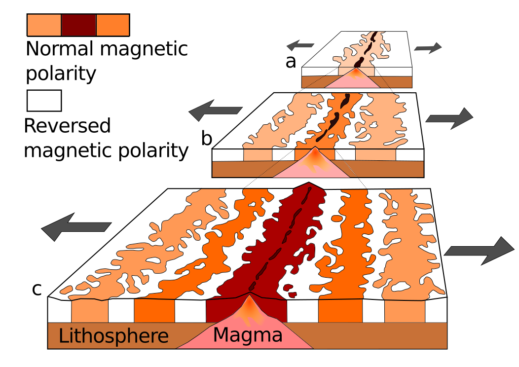 |
| Seafloor spreading at a mid-ocean ridge, recording time-changes of geomagnetic field polarity. Source: Wikimedia Commons. |
 |
| Map of the age of the seafloor based on the reversal of the magnetic field recorded in the oceanic crust during its formation at mid-oceanic ridges. Red indicates a young seafloor, whereas blue is used for the oldest oceanic crust. (Source: National Geophysical Data Center) |
Magnetic reversals are still today one of the key methods allowing rock dating (don't miss the name for it: magnetochronostratigraphy). But we know very little about the mechanisms responsible for these magnetic field changes. Computer simulations suggest that it is a natural result of feedback forces between the magnetic field and the flow in the Earth's core (see the reference to Glatzmaiers' below), similar to dynamo going tilted by its own magnetic field. It has been recently shown in this article in GRL a correlation between the distribution of tectonic plates and the frequency of magnetic reversals over geological time ("geological intervals characterized by an asymmetrical distribution of the continents with respect to the equator are followed by intervals of high reversal frequency"), suggesting a mechanical coupling between both phenomena. But the specific mechanism behind magnetic reversals and the additional information they may contain about the interior and the past of our planet remain, so far, a challenge (yet another Reto Terrícola!).
Update (2015-09): A Science News article on a recent study on core convection and the magnetic field.
Anyone thinking of the Earth as a static thing? Here is the global magnetic declination in 1492 and today: pic.twitter.com/0WjJiwDpmx— ∆ Garcia-Castellanos (@danigeos) July 6, 2015
The origin of the Earth's magnetic field
explained in 9 minutes.
References:
Vine, F., & Matthews, D. (1963). Magnetic Anomalies Over Oceanic Ridges Nature, 199 (4897), 947-949 DOI: 10.1038/199947a0
Pétrélis, F., Besse, J., & Valet, J. (2011). Plate tectonics may control geomagnetic reversal frequency Geophysical Research Letters, 38 (19) DOI: 10.1029/2011GL048784
Glatzmaiers, G., & Roberts, P. (1995). A three-dimensional self-consistent computer simulation of a geomagnetic field reversal Nature, 377 (6546), 203-209 DOI: 10.1038/377203a0
2012-02-20
Pakistan Tribune: Hunza landslide dam to be blasted on Feb. 27th
Maybe you were following the flood risk created 2 years ago by the Hunza Valley landslide in January 2010. There were fears that once the lake overflowed it would trigger a massive outburst flood (you can have a look at my previous post, focused on this phenomenon). More than 25,000 people in Gojal were stuck after the massive landslide formed a natural dam in the Hunza River, creating a lake that consumed upstream villages as it expanded. The landslide also blocked the Karakoram Highway, a vital trade link connecting the region to China.
The spillways need to be blasted (...)The district administration of Hunza Nagar made an announcement last week to blast the spillway on February 18, but put off the task till the 27th of this month.(...)Explosives will be used to blast the boulders currently obstructing the outflow of water though a spillway dug in 2010. Several unsuccessful attempts have been made in the past using controlled blasting to widen the spillway.An official said that traffic on the Gilgit-Hunza portion of the Karakoram Highway would be stopped on that day. Authorities also warned residents settled downstream to avoid venturing to the riverside. Pakistan Red Crescent society (PRCS) has deputed a team of volunteers to assist the administration in case of an emergency.
[Via The Landslide Blog]
Update 2012-03-01: Level went down by 7m after works to enlarge the spillway and the reopening by blast last monday. Good news for people living downstream: pamirtimes.net
This has been probably helped by the erosion produced by the peak discharge reached, about 50,000 cusecs (1400 m3/s).
Update 2012-05-15: Another blast of the gravel dam: Pamir Times.
2012-02-17
Megafloods, gradualism, and the birth of geology
Altai Republic, southern Siberia, close to Mongolia. All the mountains around are older than 60 million years and we are about 300 m above the Chuja River. And yet we are stepping on recent (Pleistocene) gravels! These gravels are similar to those in every river bed except for their elevation above the river and for the fact that they show no apparent stratification: good indications that they were deposited in turbulent waters at that height, only 15 thousand years ago. The problem is: considering the valley width and the slope along the river in this area (~0.6%), such high water should have moved faster than 30 m/s, implying a discharge of about 100 times the present Amazon river. This event is getting to be known as the Altai Flood (+ info in this pdf).
No meteorological event could explain such a huge water discharge, particularly in a small catchment like that of the Chuja River. Instead, Russian geomorphologists came out during the 80's with this explanation: some tens of kilometers upstream (here), a glacier blocked the Chuja River for some thousands of years and formed a large lake behind. When the ice barrier collapsed, the sudden release of the lake's water produced a gigantic outburst flood with no historical precedent. This is today the most accepted interpretation of features such as the gravels laying along the flanks of the Katun valley (e.g., Herget, 2009).
No meteorological event could explain such a huge water discharge, particularly in a small catchment like that of the Chuja River. Instead, Russian geomorphologists came out during the 80's with this explanation: some tens of kilometers upstream (here), a glacier blocked the Chuja River for some thousands of years and formed a large lake behind. When the ice barrier collapsed, the sudden release of the lake's water produced a gigantic outburst flood with no historical precedent. This is today the most accepted interpretation of features such as the gravels laying along the flanks of the Katun valley (e.g., Herget, 2009).
 |
| This picture is taken from the top of the gravel deposits, nearly 300 m above today's river level. The gravels (note their size of a few cm) are interpreted to mark the upper reaches of the flooding waters when they encountered the hill obstacle and then ran up converting kinetic energy into potential energy. Location map. Other photos of this fieldtrip here. |
But wait, doesn't all this sound a bit pre-geological? Religions often depict the Earth as being shaped by large floods and cataclysms following Creation. Is geology now acknowledging some truth in those myths?
2012-02-15
Steady-state topography during orogenesis: Erosion vs. Tectonics competition
I uploaded to Youtube a simple but interesting numerical model. It computes a constant tectonic uplift with the competing river erosion along a cross section, allowing enough time to reach two successive topographic steady states (one during uplift, another one after uplift):
This is calculated assuming constant uplift rate at the center (x=-50 to +50 km) and a 1D stream power law erosion model. Uplift rate is 1 mm/yr and stops at t=5 Myr. River erosion is proportional to slope and water discharge. Precipitation rate is constant over the entire profile. Calculations are performed under Linux with the program tAo (Garcia-Castellanos, 2007, EPSL). +info and software download here: https://sites.google.com/site/daniggcc/software/tao
As you can see, topographic growth goes on until a first steady state (with a maximum topography of ~3000 m) is reached before 5 Myr. If you look at the numbers, you'll see an equilibrium between erosion rates and uplift rates at that time. At 5 Myr uplift stops and then erosion leads to the new equilibrium: a flat topography (at 8 Myr).
Now, the question is: does steady-state topography exist in nature? And if it does, can we recognize it? In real Earth, neither climate nor tectonics are constant through time. The questions are probably too big for this small blog, but you can find some hints in this article by Willett and Brandon (2001).
Nevertheless, the notion of steady-state topography is useful to understand some basic principles of orogenesis, as Whipple (2009) showed in a very simple and elegant way. Consider these two end-member types of orogen:
Assume both orogens grow in response to the convergence of two tectonic plates, producing a constant tectonic flow Fa, and that they are eroded at a rate proportional to elevation. The red lines in the figures above correspond to a change to double erosion efficiency. With such a simple representation, it becomes clear that if erosion mechanisms become more efficient, both orogen types initially undergo an increase in erosion rate, but this will gradually decrease back to the initial erosion value (the one compensating the imposed tectonic flow, as in the animation above). The way the orogen returns to the original low erosion rate is by decreasing its elevation R.
One interesting thing is that, whereas for a fixed width, rock uplift rates return to normal after some time, the self-similar growth predicts a permanent increase in uplift rates.
And the other interesting conclusion is that the time response is controlled mainly by the erosion efficiency itself (within the approaches of the model, of course).
Simple models are generally more inspiring than the most complex ones.
References:
Whipple, K. (2009). The influence of climate on the tectonic evolution of mountain belts Nature Geoscience, 2 (2), 97-104 DOI: 10.1038/ngeo413
Willett, S., and Brandon, M. (2001). On steady states in mountain belts Geology, 30, 175-178
Steady state topography development, and other parameters of the model.
Uplift occurs between x=-50 and x=+50 km. The dashed line indicates
the topographic profile that would develop in absence of erosion.
Equilibrium topography is reached at ~4 and at ~8 Myr.
This is calculated assuming constant uplift rate at the center (x=-50 to +50 km) and a 1D stream power law erosion model. Uplift rate is 1 mm/yr and stops at t=5 Myr. River erosion is proportional to slope and water discharge. Precipitation rate is constant over the entire profile. Calculations are performed under Linux with the program tAo (Garcia-Castellanos, 2007, EPSL). +info and software download here: https://sites.google.com/site/daniggcc/software/tao
As you can see, topographic growth goes on until a first steady state (with a maximum topography of ~3000 m) is reached before 5 Myr. If you look at the numbers, you'll see an equilibrium between erosion rates and uplift rates at that time. At 5 Myr uplift stops and then erosion leads to the new equilibrium: a flat topography (at 8 Myr).
Now, the question is: does steady-state topography exist in nature? And if it does, can we recognize it? In real Earth, neither climate nor tectonics are constant through time. The questions are probably too big for this small blog, but you can find some hints in this article by Willett and Brandon (2001).
Nevertheless, the notion of steady-state topography is useful to understand some basic principles of orogenesis, as Whipple (2009) showed in a very simple and elegant way. Consider these two end-member types of orogen:
 |
| Evolution of for parameters (orogen width, erosion, topography, and rock uplift) for two simple models of orogenic growth. Left: fixed width orogen; Right: Self-similar growth. At t=0, the erosion coefficient is set to a double value (red) and to half of the reference value (green). Erosion is assumed proportional to elevation. The parameters are shown normalized. Redrawn from Whipple (2009). |
One interesting thing is that, whereas for a fixed width, rock uplift rates return to normal after some time, the self-similar growth predicts a permanent increase in uplift rates.
And the other interesting conclusion is that the time response is controlled mainly by the erosion efficiency itself (within the approaches of the model, of course).
Simple models are generally more inspiring than the most complex ones.
References:
Whipple, K. (2009). The influence of climate on the tectonic evolution of mountain belts Nature Geoscience, 2 (2), 97-104 DOI: 10.1038/ngeo413
Willett, S., and Brandon, M. (2001). On steady states in mountain belts Geology, 30, 175-178
Subscribe to:
Posts (Atom)