Showing posts with label isostasy. Show all posts

2015-07-30

Erosion in northern Spain (Ebro Basin)

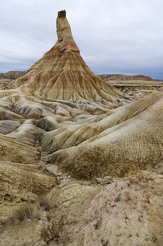
The previous post dealt with the erosion of the Ebro Basin after its colmatation with sediment, about 10 million years ago. The journal Geology has just chosen the following picture to illustrate the cover of their August volume:

Castildetierra is one of the many hills sculpted by erosion of the ancient
sediment infill of the Ebro Basin at Bardenas Reales (Navarra, Spain). 

Photo: Larrión & Pimoulier.
Location: 42.2103 N, 1.5157 W
The soft alluvial clays that make most of this hill are interbedded with harder lacustrine limestones and fluvial sandstones. The same alternation prevails over much of the Ebro Basin (NE Spain). These strata record a 19-million-year-old lake and alluvial system in the centre of an endorheic Ebro basin (84,000 km2 in area). Subsequent basin capture and drainage integration towards the Mediterranean lead to erosional features like the one in the picture.

Despite the most recent sedimentary has been removed by erosion, our study could date this major drainage change at 12.0-7.5 million years ago, based on isostatic modeling constrained with paleomagnetic data. In these badlands at Bardenas Reales (Navarra), high erosion rates have been measured in the order of millimeters per year, but how these rates link to the long-term history of the region is unclear. Other places in the basin show Pleistocene erosion rates in the order of 0.1-0.4 mm/yr, whereas our results suggest an average erosion rate since the Miocene of 0.05-0.1 mm/yr.


Summary of the scientific article in Geology: Basins formed within mountainous regions often become perfect sedimentary traps that do not drain to the sea but to internal evaporitic lakes. When they do, their sediment layers ideally record the climatic, topographic, and tectonic history of the surroundings. And when these basins eventually overtop or overfill with sediment, they are rapidly excavated by the new outflowing fluvial network, exposing excellent stratigraphic outcrops. However, this erosion often removes the uppermost basin infill, and essential information about the late basin history is lost. We have estimated the timing and elevation of the maximum infill of the Ebro basin (NE Spain) by computing the rebound of the basin in response to erosion, adopting the common idea that the Earth's rigid outer shell (the lithosphere) rests on a fluid magmatic asthenosphere in an Archimedes-type equilibrium (isostasy). We combine these calculations with existing paleomagnetic ages of the sediment basin infill. The results show that the basin became overfilled between 12 and 7.5 million years ago, and that it reached a maximum elevation of up to 750 m above present sea level. The basin has been ever since incised at a rate close to 0.1 mm/yr and has been isostatically uplifted by up to 630 m at its center. This uplift may explain why the Ebro River, opposite to other large Mediterranean rivers, does not present a deep gorge excavated within its own basin during the desiccation of the Mediterranean (Messinian salinity crisis, 5.5 million years ago).


Evolución topográfica de la Cuenca del Ebro

[Este post hace divulgación de un trabajo que acabamos de publicar en Geology
[This is outreach material about our own research, now published in Geology

Viajando entre Navarra y Lleida habrás reparado seguramente en las capas casi horizontales de sedimento, omnipresentes en la Cuenca del Ebro. Se trata de sedimento depositado en el fondo de lagos y en ríos durante el Mioceno (hace entre 24 y 5 millones de años), proveniente de la erosión del Pirineo y, en menor medida, del Sistema Ibérico y la Cordillera Costero-Catalana.

1. Vista desde la cima de San Caprasio (Zaragoza), en el centro de la Cuenca del Ebro (cubierta por las nubes). A la derecha aparecen los sedimentos calcáreos más modernos preservados en la cuenca, datados en 13.6 millones de años. Foto: DGC.
2. Bardenas Reales (Navarra). Foto: PN Bardenas.
Soft alluvial clays interbedded with harder lacustrine limestones and fluvial sandstones predominate over much of the Ebro Basin in NE Spain. In these badlands at Bardenas Reales (Castildetierra, Navarra), high erosion rates have been measured in the order of millimeters per year, but how these rates link to the long-term history of the basin is unclear. These strata record a 15-million-years-old lake and alluvial system in the centre of an endorheic Ebro basin (84,000 km2 in area). Subsequent basin capture and drainage integration towards the Mediterranean lead to erosional features like the one in the picture. Our study dates this major drainage change at 12.0-7.5 million years ago. Location: 42.2103 N, 1.5157 W
3. La roca calcárea en lo alto del
Cabezo de Castildetierra (Bardenas 
Reales, Navarra) apenas protege a 
las margas de la erosión. Esas calizas 
se formaron en los lagos que ocupaban 
la Cuenca del Ebro hace entre 36 y 10 
millones de años. Foto: Carlos Sancho

Ese sedimento contiene importantes cantidades de yeso recristalizado (CaSO4·2H2O, Imagen 4), proveniente de la disolución de yesos más antiguos en el Pirineo. La acumulación de estas rocas evaporíticas indica que ese antiguo sistema de lagos del centro de la cuenca carecía de desaguadero, es decir, era un sistema endorreico en el que todo el agua recogida acababa siendo evaporada.

4. Yeso cristalizado visible en los niveles intermedios de San
Caprasio. Unos 18 millones de años de edad. Foto: DGC 
Tras ese largo periodo endorreico, el sistema lacustre rebosó o resultó colmatado de sedimento, formándose el actual río Ebro, que ha erosionado y transportado al delta más de 30,000 km3 del antiguo relleno de la Cuenca del Ebro. Hoy, el sedimento preservado más elevado está precisamente en la zona central de la misma, en la Sierra de Alcubierre, 20 km al este de Zaragoza y a 840 m sobre el nivel del mar (Imagen 1).
¿Porqué están más altos esos sedimentos en el centro de la cuenca, si los lagos deberían ocupar la zona topográficamente más baja? ¿Y porqué no rebosaron antes los lagos hacia el Mediterráneo, si la actual divisoria de la cordillera Costero-Catalana tiene lugares de menos de 500 m de altitud?

En ausencia de deformación tectónica (las cadenas montañosas circundantes ya se habían acabado de formar), los movimientos verticales de la superficie de la Tierra están generalmente relacionados con la isostasia: La erosión de la cuenca del Ebro supuso una descarga y un levantamiento (un rebote isostático) de la litosfera terrestre, que descansa sobre el manto como si se tratara de un iceberg en el océano.
5. Hundimiento isostático que sufre la litosfera (en gris) sobre la
astenosfera fluida (blanco) cuando sobre ella descansa una carga (verde),
para 4 escenarios en los que la litosfera es progresivamente más delgada y débil.
En el escenario de una litosfera muy gruesa y rígida no se producen movimientos verticales
de reajuste. En el caso más débil, cada columna del sistema se reajusta localmente y
tiene el mismo peso si se mide hasta un nivel de compensación en la astenosfera. Autor: DGC
En nuestro artículo de esta semana, hemos calculado estos movimientos verticales de la litosfera terrestre para poder estimar el volumen de sedimento erosionado que falta en la cuenca del Ebro. Comparándolo con el volumen actualmente acumulado en el delta del Ebro, hemos podido establecer la edad en la que se produjo la colmatación, el relleno máximo de la cuenca, entre 7.5 y 12.0 millones de años, así como la altitud original que alcanzó la cuenca: 535–750 m sobre el nivel actual del mar.
6. Animation (reload page if necessary): Estimated topographic evolution of the Ebro Basin (NE, Spain) since 10 million years ago until present


7. Las cuencas endorreicas (zonas que no drenan sus aguas al mar) suelen presentar sistemas lacustres que son extremadamente sensibles a las variaciones climáticas, pues en ellos la superficie lacustre se debe adaptar para compensar la lluvia recogida con la evaporación en su superficie.

2014-06-05

Dynamic topography vs. isostasy: The importance of definitions

Fig. 1. Airy isostatic model: every column of rock above the
compensation level should have the same weight.
High topography is compensated by a mass deficit at
the base of the crust (crustal root) 
The term 'Dynamic Topography' is one of the top trending topics in Solid Earth science. It has now prevailed for more than 2 decades, but still the concept involves significant confusion. Dynamic Topography refers to a part of the elevation of the Earth surface that cannot be accounted by the classical crustal isostatic models (Pratt or Airy). But is the term referring to all mantle-sourced loads? Or only to those forces created by the dynamic flow of the mantle? Let's see first where the current confusion exactly comes from.

The term was actually coined by oceanographers to refer to the deviations of the surface of the ocean relative to the Geoid (eg., Bruce, 1968; Wyrtki, 1975). In principle, the geoid should perfectly fit the surface of the ocean, since it is an equipotential surface of the gravity field, but the flow of water adds a secondary shift of the surface, normally less than a meter. This deviation from the surface predicted for a 'static' ocean (ie., the geoid) can be detected in satellite altimetry data because the signal noise introduced by tides, waves, and wind can be removed by time-filtering. The remaining deviation from the geoid is referred to by oceanographers as 'dynamic topography' and is known to be related to the water currents in the ocean.
Fig. 2. Mean ocean dynamic topography from http://grace.jpl.nasa.gov, updated from Tapley et al., 2003).
 It measures the long-term-averaged strength of ocean currents, the 'steady-state'
circulation. 
In the 80s the term was adopted by solid-earth scientists (Hager et al., 1985, Nature). The authors did not follow the original oceanographic meaning, but instead they included 'static' forces originated within the lithosphere (such as the weight of sinking plates, or slab pull) as well as forces caused by flow in the mantle.

Mantle convection model: Mantle temperature (color shading) and flow (arrows). Lines indicate the calculated dynamic topography (blue line) and the horizontal component of plate motion (red, positive means eastward). From Liu et al., 2008, Science
This made sense at the time because there was a big questionmark (still poorly answered today) about the origin of hidden loads, the enigmatic forces needed to explain the depth of sediment accumulations next to mountain belts (see Allen's book Foreland basins, or this article pdf). Sedimentary basins next to orogens in compressional plate boundaries are formed by the isostatic sinking (subsidence) of the lithosphere due to the weight of the growing orogen. These settings became very attractive in solid-earth science not only for prospection purposes, but also because they provide an opportunity to understand how tectonic processes interact with the erosion and transport of sediment in the surface, since the sedimentary layers in such foreland basins record the tectonic evolution of the mountain belt. After many of these foreland basins were modeled, it became clear that the isostatic load of the orogen was generally insufficient to explain the amount of subsidence of the basin. But linking all the hidden load to dynamic effects is misleading, because of the presence of static forces such as the weight of a sinking plate attached to the surface (a lithospheric slab), well known since plate tectonics became mainstream. Another key to understanding the confusion is that before the widespread development of seismic tomography, everything occurring below crustal levels was far more conjectural than today. As a result, part of the Solid-Earth community used the term dynamic topography to refer to all deep-seated forces (originated below the crust) that had an effect on topography, including for instance changes in the thickness of the lithospheric mantle, or a lithospheric slab.

Fig. 3. Two static forces in balance
(weight of the books and the
counteracting human force)
Dynamic forces are added to the
static force to recover the balance
and avoid the books  from falling.
In physics, static vs. dynamic forces refer to whether the forces are in equilibrium (perfectly compensated) or not, and dynamic physical problems refer to motions involving acceleration. This is an additional source of confusion, since both the ocean flow and the Earth's mantle flow can be under steady-state flow and still inflict a constant deflection of the topographic surface, that we yet call 'dynamic'.

But sticking to the original oceanographic definition (as for example in Braun 2010), the dynamic topography of the solid-earth should restrict to the change in elevation produced by dynamic forces related to mantle viscous flow (and flow can only occur beneath the boundary layer of the mantle, underneath the lithosphere). This definition seems robust because the lithosphere is defined based on its strength relative to the underlying asthenosphere, and hence flow-related stresses are expected to be negligible above the lithosphere-asthenosphere boundary (LAB). The fact that the flow is generated by density contrasts does not mean that the forces can be mistaken for static ones, because those density anomalies are out of the rigid body being deformed (the lithosphere).

We therefore can split the observed topography OT into:
OT = CIT + LMIT + MFDT
where CIT is the crustal isostatic topography; LMIT is the Lithospheric-mantle isostatic topography (including slabs attached to the Earth's crust, or the thinning of the lithosphere); and MFDT is the sublithospheric mantle-flow dynamic topography. Note that OT-CIT (easy to calculate using global databases of crustal thickness) is often called residual topography (RT).

Following this notation, the confusion can be described as emanating from some authors referring to LMIT+MFDT (which equals RT) as the dynamic topography, instead of MFDT alone. While this RT ranges in the order of +-1 km, there seems to be no consensus yet as to how large can MFDT be, with values ranging between that same value and a few hundred meters.

Fig. 4. Global free-air gravity anomaly from GRACE. The low values (+-40 mGal) in comparison with the +- 300 mGal that are often attained in smaller regional scales shows that the crust is in overall isostatic equilibrium: the mass excess of topography at high-elevation areas is compensated by a mass deficit at the base of the crust. For this reason there is little correlation between anomaly and continents. The Hawaiian, Yellowstone, Iceland hotspots are represented by highs. Subduction zones show an asymmetrical pair of low & high anomaly. The Hudson Bay undergoes a glacial rebound in response to the deglaciation (+ info here).

Support for the smaller MFDT values comes from reasonings like this: Consider a Stokes sphere sinking or rising in a viscous fluid by virtue of its density contrast with the surrounding fluid (the viscous mantle for us). The vertical velocity of this sphere can be analytically solved and the expression obtained for the dynamic topography it produces depends on its radius a, its density contrast relative to the fluid, the depth of the sphere, and the distance R from the measuring point in the surface to the center of the sphere.
MFDT = ∆h[m] = 2*∆density * a^3 * D * (3D^2+3a^2-5*D^2*a^2/R^2) / (3*fluid_density*R^5) 
Stokes' sphere sinking in a viscous fluid. The gravity anomaly and dynamic topography it generates are linearly proportional to each other.
Because the free-air gravity anomaly produced by the same sphere (∆g) follows a similar equation, the relation between gravity and MFDT conveniently depends only on the of fluid density, to a first approach:
∆g[mGal] = 2πG * density[kg m-3] * MFDT[m]

This means that the +-40 mGal anomalies shown in the global map above should correspond to a dynamic topography smaller that 300-400 m (see P. Molnar's talk linked below).

Clearly, if we knew well the two isostatic contributions CIT+LMIT, then we would be able to attribute the rest to the flow in the mantle and learn about what happens at those depths. As Jean Braun puts it: "Mantle dynamics remain poorly constrained, but by linking mantle flow to surface topography (...) we can use the geological record to constrain the dynamics and viscosity of the mantle and the density structure that controls its flow".
The problem is that there are too many unknowns in the equation: computer models of 3D mantle flow that estimate dynamic topography rely on seismic tomographic imaging of the mantle that provide the distribution of seismic velocity anomaly but how to translate this wave velocity into lateral inhomogeneities in density and viscosity is poorly known. So, fitting the computer models to the weak available observations of dynamic topography and plate tectonic reconstructions will provide only hints on a vague combination of the velocity-viscosity and the velocity-density relationships. So, this will remain as an Earthling Challenge (a Reto Terrícola) for quite some time.

For more information, I recommend Peter Molnar's talk on youtube, Philip Allen's blog post, or Braun's paper listed below. PS: Check also this recent talk by Jean Braun on the interaction between erosion and dynamic topography.


References
  • Allen, 2010, Surface impact of mantle processes, Nature Geoscience.
  • Braun, Jean. "The many surface expressions of mantle dynamics." Nature Geoscience 3.12 (2010): 825-833.
  • Bruce, J. G. "Comparison of near surface dynamic topography during the two monsoons in the western Indian Ocean." Deep Sea Research and Oceanographic Abstracts. Vol. 15. No. 6. Elsevier, 1968.
  • Faccenna, C., Becker, T. W., Auer, L., Billi, A., Boschi, L., Brun, J.-P., Capitanio, F. A., Funiciello, F., Horvath, F., Jolivet, L., Piromallo, C., Royden, L., Rossetti, F., and Serpelloni, E.: Mantle dynamics in the Mediterranean. In press at Rev. Geophys., 2014. PDF
  • Hager, Bradford H., et al. "Lower mantle heterogeneity, dynamic topography and the geoid." Nature 313.6003 (1985): 541-545.
  • Tapley B.D., D.P. Chambers, S. Bettadpur and J.C. Ries, 2003: Large scale ocean circulation from the GRACE GGM01 Geoid. Geophys. Res. Letters 30 (22):doi:10.1029/2003GL018622
  • Wyrtki, Klaus. "Fluctuations of the dynamic topography in the Pacific Ocean."Journal of Physical Oceanography 5.3 (1975): 450-459.

2012-09-10

Watch the Lithosphere moving up and down

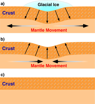
The lithosphere, the uppermost resistent layer of the Earth, rests on the fluid mantle underneath and moves up (or down) in response to weight removed from its surface (or placed on it), such as ice capes, large lakes, mountain ranges, volcanos...  
Isostatic sinking (subsidence) and
rebound (uplift) occurring when an
ice sheet forms by climate cooling
and when it is removed by climate warming.
The downwarping (isostatic subsidence)
produced by the ice accumulation in a) is
fully recovered in this process (b and c). 
My first steps into geoscience dealt with this concept called isostasy, which looked somewhat simple to a recent graduate in Physics as I was back then, since it simply applies the Archimedes Principle to the Earth's lithosphere. But this idea was just emerging in the late 19th century. And still, G.K. Gilbert was there to get it and to apply it to one of its most conspicuous scenariosLake Bonneville. 

Lake Bonneville was an enormous closed lake (meaning it had no outlet) encompassing the western half of Utah during the Pleistocene. The Great Salt Lake is a small remnant. It would be among the few largest, deepest, and highest lakes today. When its level raised to 1500 m above sea level at the end of the last glaciation, 15,000 years ago, its waters found an exit through the Red Rock pass and the lake was suddenly drained. It produced one of the largest floods ever recorded: the Bonneville Flood (see this previous post). But there was another consequence to the flood: When the lake water was released, the lithosphere under the lake moved upwards to readjust its isostatic equilibrium with the viscous mantle that underlies the Earth's crust. 

Now, do you believe this story?

2012-02-15

Steady-state topography during orogenesis: Erosion vs. Tectonics competition

I uploaded to Youtube a simple but interesting numerical model. It computes a constant tectonic uplift with the competing river erosion along a cross section, allowing enough time to reach two successive topographic steady states (one during uplift, another one after uplift):
Steady state topography development, and other parameters of the model.
Uplift occurs between x=-50 and x=+50 km. The dashed line indicates 
the topographic profile that would develop in absence of erosion. 
Equilibrium topography is reached at ~4 and at ~8 Myr.

This is calculated assuming constant uplift rate at the center (x=-50 to +50 km) and a 1D stream power law erosion model. Uplift rate is 1 mm/yr and stops at t=5 Myr. River erosion is proportional to slope and water discharge. Precipitation rate is constant over the entire profile. Calculations are performed under Linux with the program tAo (Garcia-Castellanos, 2007, EPSL). +info and software download here: https://sites.google.com/site/daniggcc/software/tao

As you can see, topographic growth goes on until a first steady state (with a maximum topography of ~3000 m) is reached before 5 Myr. If you look at the numbers, you'll see an equilibrium between erosion rates and uplift rates at that time. At 5 Myr uplift stops and then erosion leads to the new equilibrium: a flat topography (at 8 Myr).

Now, the question is: does steady-state topography exist in nature? And if it does, can we recognize it? In real Earth, neither climate nor tectonics are constant through time. The questions are probably too big for this small blog, but you can find some hints in this article by Willett and Brandon (2001).

Nevertheless, the notion of steady-state topography is useful to understand some basic principles of orogenesis, as Whipple (2009) showed in a very simple and elegant way. Consider these two end-member types of orogen:

Evolution of for parameters (orogen width, erosion, topography, and rock uplift) for two simple models of orogenic growth. Left: fixed width orogen; Right: Self-similar growth. At t=0, the erosion coefficient is set to a double value (red) and to half of the reference value (green). Erosion is assumed proportional to elevation. The parameters are shown normalized. Redrawn from Whipple (2009).  
Assume both orogens grow in response to the convergence of two tectonic plates, producing a constant tectonic flow Fa, and that they are eroded at a rate proportional to elevation. The red lines in the figures above correspond to a change to double erosion efficiency. With such a simple representation, it becomes clear that if erosion mechanisms become more efficient, both orogen types initially undergo an increase in erosion rate, but this will gradually decrease back to the initial erosion value (the one compensating the imposed tectonic flow, as in the animation above). The way the orogen returns to the original low erosion rate is by decreasing its elevation R.
One interesting thing is that, whereas for a fixed width, rock uplift rates return to normal after some time, the self-similar growth predicts a permanent increase in uplift rates.
And the other interesting conclusion is that the time response is controlled mainly by the erosion efficiency itself (within the approaches of the model, of course).

Simple models are generally more inspiring than the most complex ones.

References:

Whipple, K. (2009). The influence of climate on the tectonic evolution of mountain belts Nature Geoscience, 2 (2), 97-104 DOI: 10.1038/ngeo413

Willett, S., and Brandon, M. (2001). On steady states in mountain belts Geology, 30, 175-178